Handcoded KNN Algorithm

KNNIMAGE

Below is a hand coded (in R) K-Nearest Neighbor algorithm.  The algorithm is built to accept any 2dim dataset and will output a label vector.  I really just put this together as a way to show just how intuitive a lot of machine learning methods can be.  The R code is reasonably documented, but most readers will be able to read through without documentation as everything used is base R and the implementation is very straightforward.  ..just for fun. 🙂

set.seed(111)

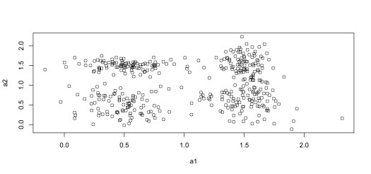
#create a basic 2 dim sample data set with four apparent cluster centers
a1<-rnorm(100,.5,.2);a2<-rnorm(100,.5,.3)
b1<-rnorm(100,1.5,.2);b2<-rnorm(100,.5,.3)
c1<-rnorm(100,.5,.3);c2<-rnorm(100,1.5,.1)
d1<-rnorm(100,1.5,.1);d2<-rnorm(100,1.5,.3)
X1<-cbind(a1,a2);X2<-cbind(b1,b2);X3<-cbind(c1,c2);X4<-cbind(d1,d2)
data_<-rbind(X1,X2,X3,X4)
plot(data_)

#add a labels column
label<-rep(0,400)
for (i in 1:400){
  label[i]<-floor((i-1)/100)
}
label<-as.matrix(label)
data<-cbind(data_,label)
colnames(data)<-c("x","y","label")

write.csv(data,file="data.csv")

Above is just code that can be used to generate a makeshift dataset with 4 apparent data centers

Quartz %d

#Import our dataset
data <- read.csv("...")

set.seed(111)
#create a distance matrix function
dmatrix<-function(d){
  n=nrow(d)
  dmat<-matrix(rep(0,n^2),nrow=n,ncol=n)
  for(i in 1:n){
    for(j in 1:n){
      dmat[i,j]=sqrt((data[i,2]-data[j,2])^2+(data[i,3]-data[j,3])^2)
    }
  }
  return(dmat)
}

#create a nearest neighbor ID function
kn<-function(i,dmat,k=5){
  x<-dmat[i,] #return the row of interest
  x<-order(x) #order the row
  return(x[2:k+1]) #return the first k entries (excluding the first)
}

#create a function to output predictions based on new data
knn<-function(data,k=5){
  n<-nrow(data)
  dmat<-dmatrix(data)
  pred<-rep(0,n)
  for(i in 1:n){
  	index<-kn(i,dmat,k=k) #extract the k nearest indices using our kn function
  	pred[i]<-names(sort(table(label[index])))[1]
  }
  return(pred)
}

#run the function and assign the output to the variable x
x<-knn(data)
cbind(data$label,x)
t<-table(data$label,x);t
#   x
#     0  1  2  3
#  0 98  2  0  0
#  1  4 92  0  4
#  2  0  0 99  1
#  3  0 13  1 86

cat("the proportion of correct classifications is: ",(t[1,1]+t[2,2]+t[3,3]+t[4,4])/sum(t),"\n")
#the proportion of correct classifications is:  0.9225

As can be seen in the preceding table, the algorithm correctly classifies most of the data points in our data set (the values on the diagonal).

Traveling Salesman Algorithm (MCMC again…)

TravelSalesman

The traveling salesman problem is super easy to understand and (partly because of the problem’s simplicity) is a staple in most computer science algorithms courses.  The problem statement says:  Given the task of traveling through n cities and the restriction that each city must be visited exactly once, can we find a travel plan that minimizes the total distance traveled? Continue reading

K-Means Clustering Algorithm

ClusterAnalysisBelow is an R implementation of a k-means clustering algorithm written recently for recreational purposes.  The algorithm will accept an arbitrary bivariate data set, x, and any integer greater than 1 (the k means) as arguments.  The algorithm uses the classic optimizing mechanism:

  1. Begin by randomly choosing k centers among the n points.
  2. Group all points to the nearest of these randomly chosen centers.
  3. Find k new centers as the average of each of the partitions created in step 2.
  4. Repeat this process until stable.

This process will result in a partition of the original data set that minimizes the sum of square distances between the original n points and the final k means.  The code includes a sample data set with 4 obvious clusters.  This is only meant as an exercise in demonstrating how intuitive this algorithm actually is.  Please defer to kmeans() for all your actual k-means clustering needs. Continue reading

Monte Carlo Markov Chain Solution to the 0/1 Knapsack Problem

MCMCBelow is an R program that will optimize a particular knapsack using the Metropolis-Hasting algorithm, a Monte Carlo Markov chain.  The beautiful MH algorithm has been a recent focus of mine and I am finding that it’s applications are basically limitless.  I’ve also posted this one to my hub. The knapsack problem (in this case, a 0/1 knapsack problem) is a classic optimization problem in computer science. Many approaches exist for solving problem, but I haven’t seen many that exceed MCMC in terms of sheer efficiency and elegance. Continue reading

Using a Genetic-esque Algorithm To Solve The 0/1 Knapsack Problem

11_genetic algorithm

Below is an example of a genetic algorithm that was coded in R as a solution to a specific 0/1 knapsack problem.  This algorithm is called a genetic algorithm because the methods it uses to maximize the value of our solution vectors are based on the types of things that occur within the reproduction of chromosomes. The basic idea behind the maximization effect in the genetic algorithm runs parallel to the basic ideas behind the reproductive mechanisms at play in survival of the fittest (SOF) type of evolutionary activity in populations.  In a population that is expanding along a survival of the fittest type of trajectory the members of the population that are the fittest for survival are also the members of the population that reproduce the most. These fit parents will give rise to offspring that contain some blend of the parent’s genetic material and through this blending of genetic material, there will be a general increase in the fitness of the offspring over the long run. That is, fit parents make fitter offspring and allowing fitter parents to reproduce more will produce a population that is increasingly fit.  The algorithm takes an initial collection of chromo- some (solutions) and uses them to create generation after generation of increasingly fit chromosomes through the action of fitness, selection, crossover, and mutation. The simulation requires ‘plyr’ and ‘Rcpp’ be installed.

Continue reading

Let’s Make a Deal Simulation

11_MontyHall
Below is an R program that can be used to run Let’s Make a Deal simulations. The function, “LMAD(switch,stay)”, takes two arguments.  Switch informs the program how many simulations you would like to run where the strategy regarding the second door is to switch to the unchosen door.  Stay informs the program of the number of simulations to run where the strategy is to stay.

Let’s Make a Deal initially baffled people due to the somewhat unintuitive result that your chances of winning always improved by switching to the unchosen door.  The intuition behind this improvement in odds is obvious when looked at mathematically, but was illusive when the problem was considered in everyday terms.  The information that is obtained when discovering that one of the three doors does not contain the prize is somewhat invisible in the case of only three doors.  However, the reason for switching would be obvious if we imagine instead that there were 1,000 doors to initially choose from and then all but two were opened revealing nothing behind them.  This would make us rightly believe that there was a very good reason for the other door not being included in the 998 that were opened and shown to contain nothing.

LMAD<-function(switch,stay,conf=.95){
#Here we set a seed for reproducibility.
	set.seed(10); trials=switch+stay

#Here we set up a vector called 'strategy' that assigns our switch or stay
#indicators.
	st=c(); for(i in 1:stay){st[i]=0}
	sw=c(); for(i in 1:switch){sw[i]=1}
	strategy=c(st,sw) 

#Vector 'x' is repeatedly sampled from in order to determine whether our
#first choice contained the winning prize.
	x=c(0,0,1)

#Here we repeatedly sampling the vector 'x' and place the sampled element
#into the vector 'u'.  This simulates the first guess in the game. The vector
#'u' stores whether or not we chose the door with the prize ('1') for game i.
	u=c(); for(i in 1:trials){u[i]=sample(x)[1]}

#Here we populate the vectors 'sw' and 'st' with the outcomes of the second
#part of the game.
	for(i in 1:trials){
	#If our initial guess contained the prize and our strategy was to switch
	#we would certainly lose because the two remaining doors are empty.
		if (u[i]==1 && strategy[i]==1){sw[i]=0; st[i]=0}
	#If our initial guess contained the prize and our strategy was to stay
	#we would certainly win because the choice we are staying with is the
	#winning choice.
		else if (u[i]==1 && strategy[i]==0){sw[i]=0; st[i]=1}
	#If our initial guess did not contain the prize and our strategy was to
	#switch then after Monty revealed the other losing door we would switch
	#to the remaining door, which is the winner.
		else if (u[i]==0 && strategy[i]==1){sw[i]=1; st[i]=0}	
	#If our initial guess did not contain the prize and our strategy was to
	#stay we would certainly lose because the choice we are staying with is a
	#losing choice.
		else if (u[i]==0 && strategy[i]==0){sw[i]=0; st[i]=0}
		}

#The vector 'sw' contains 1's for all of the games we won under the switch
#strategy and the vector 'st' contains 1's for all of the games we won under
#the stay strategy.  Using these we can calculate our switch and stay win rates.
	switch_wins<-sum(sw)/switch; stay_wins<-sum(st)/stay

#Here we produce 95% lower and upper bounds on our percentage of wins.
	lower_switch<-switch_wins-1.96*sqrt((switch_wins*(1-switch_wins))/switch)
	upper_switch<-switch_wins+1.96*sqrt((switch_wins*(1-switch_wins))/switch)
	lower_stay<-stay_wins-1.96*sqrt((stay_wins*(1-stay_wins))/stay)
	upper_stay<-stay_wins+1.96*sqrt((stay_wins*(1-stay_wins))/stay)
	switch_CI=c(lower_switch,upper_switch)
	stay_CI=c(lower_stay,upper_stay)

#Here we output the results.

cat("Number of Games:",trials,"\n")
cat("-------------------------","\n")
cat("Number of switches:",switch,"\n")
cat("Number of wins when switching",sum(sw),"\n")
cat("95% CI for wins when switching:",switch_CI,"\n")
cat("-------------------------","\n")
cat("Number of stays:",stay,"\n")
cat("Number of wins when staying",sum(st),"\n")
cat("95% CI for wins when staying:",stay_CI)
}


The Buffon’s Needle Problem

Attached is a short write-up on the very interesting geometric probability problem commonly referred to as the Buffon’s Needle problem.  The solution gives a general outline for a Monte Carlo method of approximating pi. neato!Buffons Needle\

An R implementation of the monte carlo simulation is:

#Enter the desired number of trials as n

Buffon_Needle<-function(n){
	L=2;D=L;

	thetas<-c(rep(0,n))
	for(i in 1:n){thetas[i]=runif(1,0,pi/2)}

	X<-c(rep(0,n))
	for(i in 1:n){X[i]=runif(1,0,L/2)	}

	COS<-c(rep(0,n)); COS=cos(thetas)
	Compare<-c(rep(0,n))
	Compare=(X/(2/L))
	Crossover<-c(rep(0,n))
for(i in 1:n){
if(COS[i]>=Compare[i]){Crossover[i]=1}
if(COS[i]<Compare[i]){Crossover[i]=0}
	}
Total=sum(Crossover)
Pi_Est=(2*n)/Total

cat("For ",n," trials the estimate of pi is: ",Pi_Est)
}
########################################

Buffon_Needle(100)

A SAS implementation of the monte carlo simulation is:

%macro Buffon_Needle(n=);
%let D=2; %let L=2;
 
data BN;
do i=1 to &n;
     angle=rand("Uniform",0,3.14159/2);
     X=rand("Uniform",0,&D/2);
     COS=cos(angle);
     L=&L;
output;
end;
 
data BN; set BN;
if(COS >=(X/(2/L))) then Cross = 1;
else Cross = 0;
 
proc sql;
create table Results as
select (sum(t1.Cross)) as Total_Crosses
from work.BN t1;
quit;
 
data Results; set Results;
n=&n;
pi_est = (2*&n)/Total_Crosses;
 
run;
 
%mend;
 
%Buffon_Needle(n=1000000);

Math 63 HW #6

math-063

For next Saturday (October 12th), please do all of the odd problems from sections 4.4, 4.5, 4.6, 4.7, & 4.8.  Remember that your Exam 1 corrections are also due next Saturday (October 12th).  In order to receive partial credit for the problems that you missed, you will need to rework the missed problem and bring them in on a separate sheet of paper during next weeks class.  Have a great week!